Clust&See Documentation

Once installed, the user can start/stop the plugin using the Start and Stop entries in the menu Plugins->Clust&See.

Once started, the plugin opens a new tab named “Clust&See” in the Control Panel (left hand Cytoscape panel). This panel will be referred to as the “Clust&See Panel” below. The plugin also opens a new panel named “Partition Details” in the Data Panel (bottom panel). Finally, when a partition(s) has been generated, the plugin will create new panels in the Results Panel (right-hand Cytoscape panel).

All those panels will be described in detail below.

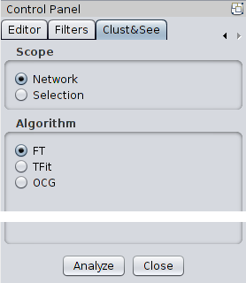
The Clust&See Panel in the Control Panel describes the parameters required to generate a partition. These elements are described below:

Scope

First, the user must select the scope on which to apply the plugin’s actions. There are two choices: Network or Selection. The Network option will apply the partitioning method to the whole network (in the currently selected view) while the Selection option will apply it only to those nodes that are currently selected in the network. Note that this option considers only the selected nodes and will, therefore, retrieve only the edges between those nodes to create the network to be analyzed.

Clust&See should only be used for the analysis of undirected networks.

Algorithm

Clust&See offers several algorithms to partition a network. All have been published and are succinctly described below:

• FT (see [1]): This algorithm produces strict partitions (no overlapping clusters) and has no optional parameters.
• TFit (see [2]): This algorithm produces strict partitions. The optional parameter ‘alpha’ is a variation of the modularity formula described in [2]:

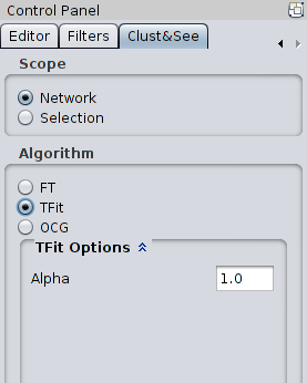
      mod = 2 * m * Aij - di * dj

With the alpha parameter:

      mod = 2 * *alpha  * m * Aij - di * dj / alpha

When alpha = 1, the modularity remains the one described in [2]. When 0 < alpha < 1, the partition results in smaller clusters since the optimal modularity is reached earlier than when alpha = 1. Note that alpha >1 and alpha < 0 are not allowed.

• OCG (see [3]): This algorithm produces overlapping partitions. It has several optional parameters that require expert knowledge of the network partitioning domain, which is why default options are proposed to the user. However, the expert level options are available if needed.

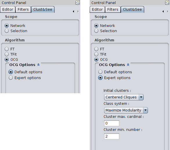
These options are:

• Initial clusters: the type of initial cluster that will be used. Possibilities are “Centered Cliques”, “Maximal Cliques” and “Edges”. See [3] for more details.
• Class system: the method for detecting optimized clusters. Possibilities are “Maximize Modularity” and “Final Class”.
• Cluster max. cardinality: set an upper limit to the number of nodes a cluster may contain. When this option is set to 0, no limit is set.
• Cluster min. number: set a lower limit to the number of final clusters the algorithm may return.

Analysis

When all the parameters have been chosen, the user may click on the “Analyze” button at the bottom of the panel to launch the clustering.

Note: If the chosen network/selection contains more than 5000 nodes, a warning will be displayed. This warning informs the user that making partitions on a network of this size:

• may lead to a very large number of clusters that will be difficult to analyze.
• may result in very long computation times (especially for the OCG algorithm) or memory issues if the computer is not sufficiently powerful or if the memory settings on the JVM (Java Virtual Machine) have not been correctly customized. The comparison of the performances of each algorithms tested on networks of different sizes is provided in the Supplementary Information file.

To work around these issues, we suggest using the “Build Neighborhood Network” function (see below) to produce a smaller network centered on the nodes of interest. The user can also use alternative clustering methods, either in-house, or through the ‘Linkcomm’ R package [4] producing compatible output files that can be loaded in the Clust&See Cytoscape plugin.

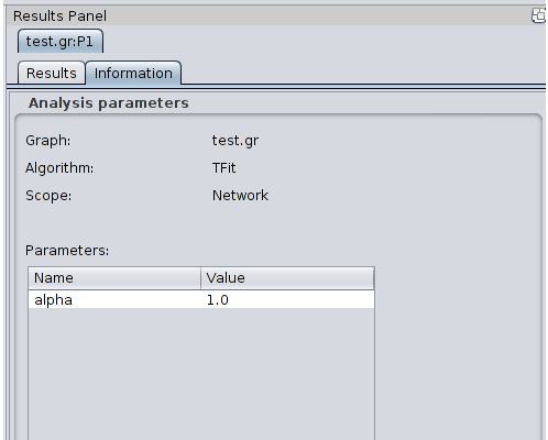
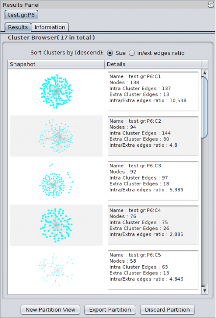
Once a partition has been produced, Clust&See displays a summary of the partition and the global quotient graph (a graph showing the edges connecting the clusters).

3.1 Partition Summary

For each computed partition, Clust&See displays a new panel with the name of the partition in the Cytoscape Results Panel (right hand side panel). This name is the network name followed by the suffix “:Px” where ‘x’ is an increasing index representing the partition number. Hence, the first partition produced on the network named “TestNetwork” will be named “TestNetwork:P1” while the second one will be named “TestNetwork:P2”.

The Results Panel of a partition contains the following elements:

• A  tab named “Information” that contains the various parameters (Network, scope, algorithm optional parameters...) used to produce the partition.

• A tab named “Results” containing a table listing the discovered clusters and, for each of them:

** An image of the cluster network

** The name of the cluster. The name of a cluster is the name of the partition followed by the suffix “:Cx” where ‘x’ is an increasing index representing the rank of the cluster. Since the clusters are ordered by their size (number of nodes they contain), the largest cluster will be named with the suffix “:C1” while the second largest cluster will be named with the suffix “:C2” and so on.

** The number of nodes in the cluster.

** The number of Intra Cluster Edges: the number of edges between nodes of the cluster. This number can differ from the edge number if loop edges (self-interactions) exist in the cluster.

** The number of Extra Cluster Edges : the number of edges in the network between nodes in the cluster and nodes outside the cluster.

** The ratio of edges between nodes within the cluster over edges between nodes of the cluster and nodes in other clusters (Intra/Extra edge ratio).

Note that the list of clusters can be classified by cluster size or by in/ext edges ratio.

• A “New Partition View” button that generates a new view of the complete partition (quotient graph).
• An “Export Partition” button that exports the partition to a file. See Export/Import below for more details.
• A “Discard Partition” button that removes all the information related to this partition.

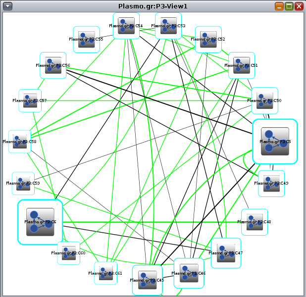
3.2 Quotient graph

At the end of the analysis, Clust&See creates a new view containing the discovered clusters represented as metanodes. Nodes representing a cluster (hereafter referred to as metanodes) are represented as cyan bordered, white square nodes with a special icon at their centre. When there are less than 50 clusters, these are represented as a circle:

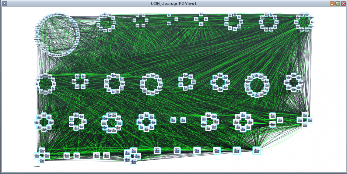
If there are more than 50 clusters, these are arranged using Cytoscape’s Group Attribute Layout, ordered by cluster size (CnS:Object Number):

In the newly created view, the metanodes may be connected by two kinds of edges (hereafter referred to as metaedges):

• black metaedges: these metaedges summarize the analyzed network edges between the nodes that are members of the two clusters. The width of the metaedge is proportional to the number of edges it summarizes. Black metaedges can also be displayed between a metanode and a single node. In such cases, they summarize the edges existing between the single node and the nodes in the cluster.
• green metaedges: these metaedges indicate that the two connected clusters share one or several nodes. These green metaedges exist only if the clustering algorithm leads to overlapping clusters (e.g. OCG). The width of the metaedge is proportional to the number of shared nodes. Green metaedges can also be displayed between a metanode and a single vertex. In such cases, they simply indicate that the node is a multi-classed member of the cluster.

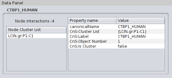
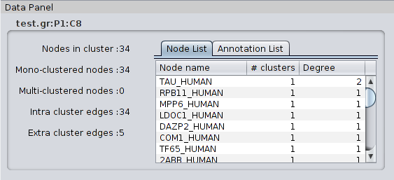
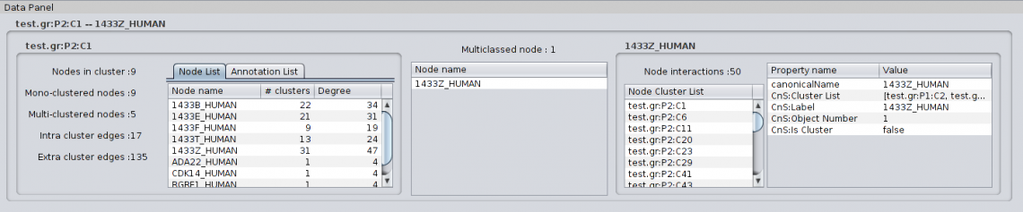
Clust&See offers several functions to help in the analysis of the computed partition.

4.1 Detailed information on objects

Selecting any object shown in a view generated by Clust&See causes detailed information about this object to be shown in the Partition Details tab located in the Cytoscape Data Panel (bottom panel). Objects can be selected from a view (nodes, edges, metanodes, metaedges) or from the cluster list in the Results Panel (clusters). Note that selecting a metanode automatically selects the corresponding cluster in the cluster list. Similarly, selecting a cluster in the cluster list automatically selects the corresponding metanode in all open views where it is present. In addition, selecting a cluster or a metanode automatically selects all the nodes of the cluster in all the views where they are present (including the original network view).

4.1.1 Node details

When selecting a node, the Partition Details tab shows the following information:

4.1.2 Cluster details

When selecting a metanode/cluster in the Cluster list of the Results Panel, the Partition Details tab shows the following information:

The Annotation List tab contains the list of annotations associated with the cluster. See the Cluster Annotation section below for more details.

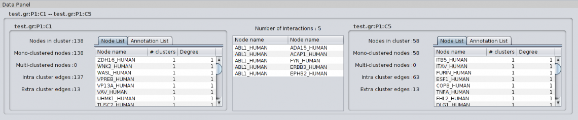
4.1.3 Black metaedge details

When selecting a black metaedge, i.e. a metaedge summarizing the connections between two clusters or between a cluster and a single node, the Partition Details tab shows the following information:

For Cluster to Cluster metaedge:

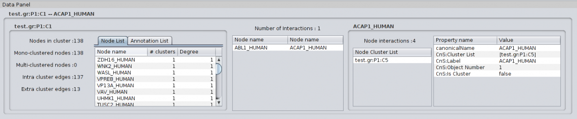
For Cluster to Protein metaedge:

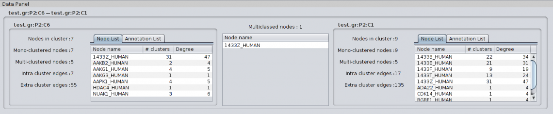
4.1.4 Details on green metaedge

When selecting a green metaedge, i.e. a metaedge indicating overlapping clusters/multiclassed nodes, the Partition Details show the following information:

For Cluster to Cluster metaedge:

For Cluster to Protein metaedge:

4.2 Customized views

When analyzing a partition, it is often necessary to focus on sub-groups of clusters. To facilitate this kind of analysis, Clust&See allows the creation of customized views of the different clusters.

When selecting a cluster in the Results Panel cluster list, several additional buttons appear at the bottom of the list:

• New Cluster View: this button adds the cluster metanode to a new, empty view.
• Add Cluster to View: this button adds the cluster metanode to the currently selected view.
• New Cluster Network View: this button adds the entire cluster network to a new empty view.
• Add Cluster Network to View: this button adds the entire cluster network to the currently selected view.

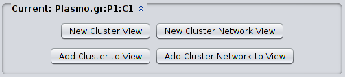
Using these four buttons, the user can produce a suitably customized view for analysis.

Any views generated as described above can be further manipulated as follows:

• Add all edges: Right-clicking on a metanode or node opens a contextual menu with the entry Clust&See->Add all edges. This action will add all the edges/metaedges that connect the nodes/metanodes present in the view.
• Expand cluster: Right-clicking on a metanode opens a contextual menu with the entry Clust&See->Expand cluster. This action will replace the metanode by the cluster network it represents in the current view. All edges/metaedges connecting the cluster’s nodes to the rest of the nodes/metanodes in the view will be added.
• Compress cluster: Right-clicking on a node opens a contextual menu with the entry Clust&See->Compress cluster. This action will replace the node by the cluster(s) it is a member of. All nodes belonging to the same cluster(s) will also be removed from the view.

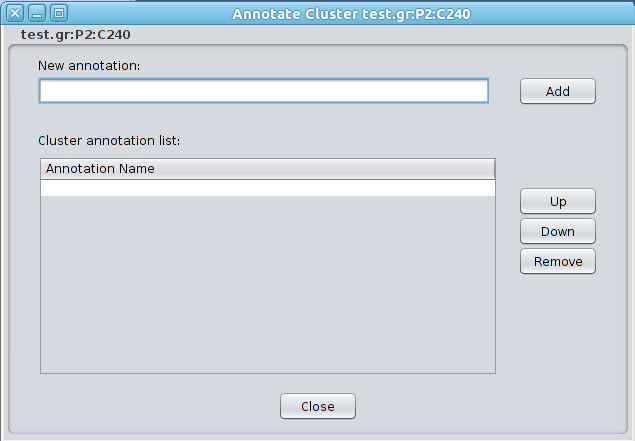
Note that if the selected node is a member of several clusters, Clust&See will only display as metanodes those clusters that already have at least one member visible in the current view. If the selected node is the only member of a given cluster currently visible, then that cluster will not be shown as a metanode. The metaedges connecting the new metanode(s) to the rest of the nodes/metanodes in the view will be added.

4.3 Cluster annotation

Once a partition has been analyzed, it is often necessary to annotate clusters in order to save the conclusion of the analysis. Clust&Sees offer the option of adding one or several annotations to a cluster and to its nodes.

Right-clicking on a node or metanode opens a contextual menu with the entry Clust&See->Annotate Cluster. Choosing this option opens the Annotate Cluster frame where annotations can be entered:

Note: this action is not available on multi-classed nodes since they are members of several clusters.

Annotations assigned to a cluster are stored at the cluster level (the Partitions Details panel contains a specific tab to display these annotations, see the “Detailed Information on Object” section above). Annotations are also inherited by the cluster’s member nodes.

4.4 Exiting Clust&See

To stop using Clust&See you can simply use the menu “Plugins -> Clust&See-> Stop”. This will close all the windows and views related to your work with Clust&See. All the results and customization you may have produced will be lost.

Note that saving the Cytoscape session will not save the Clust&See environment. In order to save your work, you have to save your partition by exporting it to file. You will then be able to re-use the exported partition in a later session.

To have details on how to export results, see the section below “Exporting/Importing partitions”.

5.1 Exporting partitions to file

Clust&See partitions can be exported to text files. The partition is exported along with its parameters (network name, scope, chosen algorithm...). These details are easily readable as headers at the beginning of the file. Global partition statistics (number and cardinality of each cluster) and cluster annotations are also exported. The exported files have the “.cns” extension.

To export a partition, click on the “Export Partition” button located in the Results Panel at the bottom of the desired partition cluster list.

5.2 Importing partitions from file

Partitions can be imported into Clust&See if they are described in a suitable formated file (see below for the file format). Files imported as Clust&See partitions into Cytoscape can come from the Clust&See export partition function (see above) but also from files built by external partition tools or scripts. Currently, the R package “Linkcomm” (Kalinka and Tomancak, 2011, http://cran.r-project.org/web/packages/linkcomm/index.html), in which the LinkCommunities (Ahn et al., 2010) and OCG (Becker et al., 2012) algorithms are implemented, provides output files of the produced partitions that can be imported into Clust&See.

If you want to visualize the result of your own partitioning algorithm into Clust&See to take advantage of its visualization features, let your tool or script produce a file describing the partition in the format described below.

In order to import a partition, load the network used to produce the partition into Cytoscape using standard load features, then click the “Import Partition” action in the “Plugins->Clust&See” menu and select the appropriate partition file (.cns file). The imported partition will behave exactly as if it was produced by Clust&See algorithms.

5.3 Partition file format

In order to be imported into Clust&See, a partition must be described in a file with the “.cns” extension, containing the information described below. First we will describe the required information, then we will detail the optional information.

5.3.1 Required information

The partition file must start with the following line:

#ClustnSee analysis export

The following lines must describe the clusters composing the partition. The first line of a cluster description starts with the string “>ClusterID:”, followed by the cluster ID followed by the characters “||” (the cluster ID must be an integer). Any annotations the cluster has follow on the same line and are separated by the “||” character. Finally, the names of the nodes that form the cluster are listed below, one node name per line. For instance, the cluster with ID “1”, consisting of nodes “nodeA”, “nodeB” and “nodeC”, and annotated with “Function1” and “Function2”, will be described as follows:

>ClusterID:1||Function1||Function2||

nodeA

nodeB

nodeC

Annotations are optional. If the cluster has no annotations, its description will be:

>ClusterID:1||

nodeA

nodeB

nodeC

A partition’s clusters are given one after the other in no particular order. What follows is an example of a minimal partition description (two clusters with  3 nodes each and no annotation):

#ClustnSee analysis export

>ClusterID:1||

MYC_HUMAN

SMAD3_HUMAN

SNW1_HUMAN

>ClusterID:2||

B4GT3_HUMAN

SAT1_HUMAN

CA103_HUMAN

5.3.2 Optional information

Clust&See can also import meta-data associated with clusters. These meta-data include:

The algorithm name. This information can be provided by the header “#Algorithm:” (followed by the algorithm name)

The parameters of the algorithm. Each parameter can be provided by the header “#Parameter:” followed by the parameter name, the equals sign (“=”) and the parameter value.

Scope of the partition can be provided by the header “#Scope:” and followed by any string describing the used scope. If a sub-network has been used to produce the partition, it is possible to provide the list of the used nodes and edges thanks to the headers “#NodeInScope:” and “#EdgeInScope:” (one node per line and one edge per line).

The above information will be imported in Clust&See and associated with the partition. It will be available in the “Information” tab next to the partition’s “Result” tab. Moreover, it is possible to insert arbitrary information in the file using the comment sign ”#”. Those lines (if not Clust&See headers) will be ignored during the import.

Below you will find complete examples:

• Example of export of partition produced by the ‘TFit’ algorithm with parameter ‘alpha=1’ on the whole “LCIN_clean.gr” network:

#ClustnSee analysis export

#Algorithm:TFit

#Network:LCIN_clean.gr

#Scope:Network

#Parameter:alpha=1.0

>ClusterID:1||

MYC_HUMAN

SMAD3_HUMAN

SNW1_HUMAN

>ClusterID:2||

B4GT3_HUMAN

SAT1_HUMAN

CA103_HUMAN

• Example of export of partition produced by ‘MyAlgo’ algorithm with parameters ‘MyParam1=1.0’ and ‘MyParam2=centered’ on a sub-network of the “LCIN_clean.gr” network:

#ClustnSee analysis export

#Algorithm:MyAlgo

#Network:LCIN_clean.gr

#Scope:Selection

#Parameter:MyParm1=1.0

#Parameter:MyParm2=centered

#NodeInScope:MYC_HUMAN

#NodeInScope:SMAD3_HUMAN

#NodeInScope:SNW1_HUMAN

#NodeInScope:B4GT3_HUMAN

#NodeInScope:SAT1_HUMAN

#NodeInScope:CA103_HUMAN

#EdgeInScope:MYC_HUMAN SMAD3_HUMAN

#EdgeInScope:SMAD3_HUMAN SNW1_HUMAN

#EdgeInScope:MYC_HUMAN SNW1_HUMAN

#EdgeInScope:B4GT3_HUMAN SAT1_HUMAN

#EdgeInScope:B4GT3_HUMAN CA103_HUMAN

#EdgeInScope:SAT1_HUMAN CA103_HUMAN

#EdgeInScope:MYC_HUMAN B4GT3_HUMAN

>ClusterID:1||

MYC_HUMAN

SMAD3_HUMAN

SNW1_HUMAN

>ClusterID:2||

B4GT3_HUMAN

SAT1_HUMAN

CA103_HUMAN

Clust&See offers several extra functions that are described below.

6.1 Search for Node Clusters

This feature is available from the menu Plugins->Clust&See. The user can enter a node name and retrieve the list of the clusters the node belongs to. This list is not restricted to a specific partition. If several partitions have been produced on the same network, the list of clusters retrieved from a node will contain clusters from the various partitions.

Each entry in this cluster list can be selected, causing the corresponding cluster and metanode to be selected in the currently open views and in the Results Panel, making it easy to locate them.

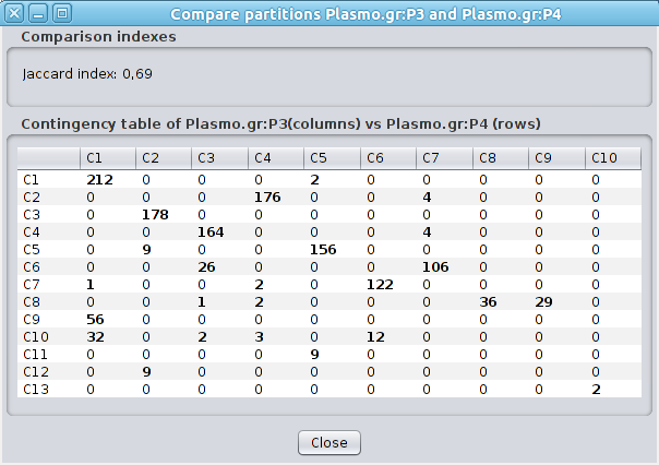
6.2 Compare Partitions

This function is available from the menu Plugins->Clust&See. It can compare two partitions computed on the same network by analyzing the dispersion of the nodes between the clusters of the two partitions. The Jaccard index between the partitions is computed and a contingency table is displayed. In this table, the columns are the clusters of the first partition and the rows are the clusters of the second. The number at the intersection of a column and a row corresponds to the number of nodes shared by the two corresponding clusters.

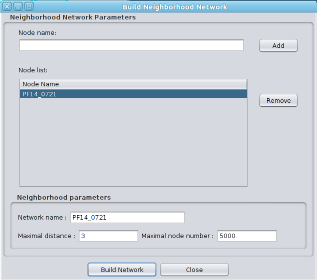
6.3 Build Neighborhood Network

As described below, Clust&See warns the user if the network/selection used for a partition analysis is too large. Launching an analysis on such a network/selection may lead, at best, to unmanageable results (too many clusters) and, at worst, to memory issues or very long computation times.

Clust&See offers the user the choice of extracting sub-networks of interest from the complete network. To do so, the user can use the “Build Neighborhood Network” feature available from the Plugins->Clust&See menu.

One or several nodes can be chosen as a starting point. The sub-network will then be extended to the nodes directly connected to the chosen nodes and, subsequently, to the nodes directly connected to those and so on until a user-defined distance limit is reached.

The user can specify:

• The maximal distance between the nodes of the final sub-network and the starting nodes (i.e. the maximal degrees of separation allowed between a node of the sub-network and the starting nodes ).
• The maximal number of nodes the final sub-network may contain.
• The name of the final sub-network.

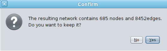
The process stops as soon as one of these conditions is met (max number of nodes exceeded or maximal distance reached) and a view is created showing the resulting sub-network. The user can then keep this network, or change the parameters and try again.

Partition analyses can be carried out on the resulting sub-network in exactly the same way as on the parent network.

[1] Alain Guénoche (2011). Consensus of Partitions: a Constructive Approach, Advances in Data Analysis and Classification 5(3):215-229. DOI: 10.1007/s11634-011-0087-6

[2] Philippe Gambette & Alain Guénoche (2011). Bootstrap Clustering for Graph Partitioning, RAIRO-Operations Research 45(4):339-352. DOI: 10.1051/ro/2012001

[3] Emmanuelle Becker, Benoît Robisson, Charles E. Chapple, Alain Guénoche & Christine Brun (2012). Multifunctional Proteins Revealed by Overlapping Clustering in Protein Interaction Network, Bioinformatics 28(1):84-90. DOI: 10.1093/bioinformatics/btr621

[4] Alex T. Kalinka & Pavel Tomancak (2011). Linkcomm: an R package for the generation, visualization, and analysis of link communities in networks of arbitrary size and type, Bioinformatics 27(14):2011-2012. DOI: 10.1093/bioinformatics/btr311